An advanced question - sampling an oscillator's signal for analysis

[dnessett]

When I first turn on the oscillator, my frequency counter shows 9,999,995Hz or thereabouts. As the oscillator warms up it reaches 9,999,999.5Hz.

Oops, I didn't pay enough attention to what you said there. The frequency change during warm up should be in the hundreds of hertz (it's 310Hz low when cold at 20°C ambient on my one), so that was a giveaway.

The HP5335A frequency error sounds like a fault rather than a calibration issue.
As you mentioned, the first thing to try would be an external reference.
I think that the HP5335A normally used a 10811 OCXO, which has a hole on the top for the frequency adjustment trimmer capacitor in it, but this will not adjust it by 150Hz.
The 10811 that I have is about 210Hz low when cold at 20°C ambient, so if your one is 150Hz low it might be worth checking if the oven is heating up - if it's there at all!

I took off the cover of the HP5335A and powered it up. It does indeed have a 10811 OCXO. After 1/2 hour there was no noticeable warmth coming from the exterior of the 10811. So, either it is busted, or something else is wrong (e.g., power not getting to it).

Right now fixing it will have to take a back door seat to building the MV89 enclosures. Did you happen to replace the fan in your HP5335A? If so, which model did you use? Mine is using a DC version of the original Pabst fan, which sounds like a small refrigerator.

[FriedLogic]

I don't have that counter, just the oscillator - this thread has some info if you've not already seen it:
https://www.eevblog.com/forum/testgear/hp-5335a-timer-counter-anything-i-should-know/

If you get to looking at the oscillator, there are various versions of the manual and other info online, such as:
http://ftb.ko4bb.com/getsimple/index.php?id=manuals&dir=HP_Agilent/HP_10811_Crystal_Oven_Oscillator
The thermal fuse and its connections often cause problems, so if the power is getting to it that might be a good place to start.

[Gerhard_dk4xp]

The MV89A that I have on my table definitely needs a +/- 5V tuning voltage.
I also have one that stops oscillating when Vtune > 0.5V. It seems they
drift down over time.

I had about 50% loss with my Chinese MV89As.
They have all a 20 year hot life behind them and are removed from their
boards in a most cruel way. There are lots of scars to prove that.

The MTI-260 also seem to have a lot of subtypes.
I'm just doing a PLL to lock all of them to an incoming reference frequency.

[dnessett]

One piece of design I need for the enclosure is an interface between the HP11729C Freq-Cont X-Osc output and the MV89A adjust input. This interface must convert the +/- 10 V swing of the Freq-Cont X-Osc output to the 0-5 V swing required by the adjust pin on the MV89A.

I came up with a simple divider network to achieve this conversion, shown in Figure 1

Figure 1 -

The 470 resistor divider pair converts +/- 10 V to +/- 5V. Using the 5V reference provided by the MV89A, the 10K resistor divider pair converts this swing to 0-5 V (in theory). I breadboarded this circuit and found that the actual swing is 1.06V - 4.3V. This reduced breadth is due to the actual voltage produced by the Freq-Cont X-Osc circuit when driving the interface. Instead of +/- 10 V, the range observed on the Freq-Cont X-Osc input was: -6.1V -> +7.2V. Since the output impedance of Freq-Cont X-Osc is specified as 100 ohms and it is driving ~940 ohms, this is a little surprising.

However, the circuit is not a simple passive network, because the MV89 Ref connection to the 10K resistor divider has an output impedance of 100 ohms (see previous message). I decided not to pursue a network analysis of the circuit, since the measured swing is sufficient to drive the MV89A adjust pin.

The SPDT switch allows the adjust pin to be driven either by the Freq-Cont X-Osc line or by a 2.5V constant voltage derived from the Ref pin. This means the MV89A can be used either as a reference oscillator in an HP11729C phase detector configuration or as a DUT analyzed by the HP11729C in a frequency discriminator configuration.

I would welcome thoughts about how to test this circuit with the HP11729C to insure it can keep the MV89A in quadrature with another oscillator over long time intervals when using a phase detection configuration.

[dnessett]

If you get to looking at the oscillator, there are various versions of the manual and other info online, such as:
http://ftb.ko4bb.com/getsimple/index.php?id=manuals&dir=HP_Agilent/HP_10811_Crystal_Oven_Oscillator
The thermal fuse and its connections often cause problems, so if the power is getting to it that might be a good place to start.

Thanks for the pointers to the manuals for the 10811. Now that I have an enclosure built for one of the MV89s, I need to get the HP5335A repaired. I started with recalibrating the two adjustable power supply voltages. The 3.1 supply was off, but I was able to get it back into range. However, the 15.7 power supply was at 15V and I could not get it to 15.7 V by adjusting the controlling pot. I suspect the HP11811 might be causing the problem, so I plan to take it out of the 5335A and troubleshoot it.

However, the power supply is connected to it by an edge connector. I thought about using a alligator clip to attach power by clipping it to the pad for that purpose, but am concerned that it will slip and put 20V onto some other pad, thereby damaging the device.

Do you have any suggestions? Is there a way to test the thermal fuse and connections without applying power to the 10811? If not, are mating connectors for the edge connector widely available (eBay or perhaps an electronic parts distributer)? How do you power your 10811?

[Gerhard_dk4xp]

The mating plug is

EDAC 305-030-520-202

That's what is printed on it. I can't find where I have ordered them, at least not quickly.
Probably Mouser or Digi Key.

I'm just doing version 2 of my OCXO support board. It hosts one of 10811A, MV89, MTI260
or CVHD-950 or ECOC2522, KVG O-30-ULPN-100M, KVG O-40-ULPN-100M for 100 MHz.

There is a Xilinx Coolrunner2 that creates a 1pps out and that has a dual Flipflop PFD.
The Oven can be synchronized to an incoming reference frequency or an incoming 1pps.
There is also a doubler for 5 -> 10 MHz if needed.

This is V1:
<     https://www.flickr.com/photos/137684711@N07/30952252115/in/album-72157662535945536/     >
<     https://www.flickr.com/photos/137684711@N07/30952263115/in/album-72157662535945536/     >
It used a ring mixer as phase detector. That could not work for 1pps.

But this is still work in progress.

regards, Gerhard

[dnessett]

If you get to looking at the oscillator, there are various versions of the manual and other info online, such as:
http://ftb.ko4bb.com/getsimple/index.php?id=manuals&dir=HP_Agilent/HP_10811_Crystal_Oven_Oscillator
The thermal fuse and its connections often cause problems, so if the power is getting to it that might be a good place to start.

Instead of trying to fix the HP10811, I decided to buy one from eBay and replace the one that came with the instrument. This fixed the problem. By tweeking the frequency adjust screw on the new 10811, I got the HP5335A to measure one MV89A oscillator frequency to within .01Hz of 10 MHz. Also, the new 10811 is warm to the touch after 10-15 minutes, whereas the old one did not warm up at all.

Of course, in effect I am using the MV89A as a calibration oscillator, so there is no guarantee that the HP5335A is actually calibrated properly. But at least it should be possible to get within 1-2 Hz of an accurate measurement.

In regards to the HP10811, I did buy a connector, so at some future point I could attempt to fix it. However, I was already sidetracked by trying to get the  HP5335A to work properly. I didn't want to get sidetracked on a sidetrack. My goal is measuring phase noise, which now, after building enclosures for the other 2 MV89As, is within reach.

[jpb]

I have an MV89 I got from China years ago and it seems to work fine (though I don't have anything that will measure its phase noise though.

The main issue with them I seem to remember for Time Nuts postings is that the 10MHz devices are frequency doubled 5MHz devices:

https://www.mail-archive.com/time-nuts@febo.com/msg58269.html

The reliability issue is to do with a capacitor going bad but that shows up as a low level output I think.

It will be interesting to see what your measurements show.

Thanks for the info, jpb.

Given your experience with the MV89, I have a question. When I ran one of the MV89s for an hour or so, I noticed it became quite hot. I am still able to pick it up and hold it my hand, but it is on the borderline of that. When you were working with yours, did you have a heatsink on it? If so, how did you attach it (as there are no screw holes for this purpose on the top)?

Sorry, I've only just seen this and now it is rather too late to reply!
Just for the record, my MV89 did not have a heat sink and it did get warm but almost all OCXOs do - in fact some get quite hot. This is not that surprising as the temperature of the crystal is around 70C or more, an OCXO that is specced to operate up to 70C must keep the crystal at some temperature above that as it has no means of cooling only heating.

On the subject of the 10811 - I had one which was broken, (weird waveform). I managed to mend it using the repair manual which is very good but then I was doing one last probe of all the voltages and managed to blow up one of the transistors. I replaced it with one I had but it was not the right specs. The original type is unobtainable but recently I got round to ordering a similar part but it has been a couple of years and one house move since I last worked on it so I'm going to have to start over when I have time.

I'm looking forward to seeing how your phase noise measurements go dnessett.
I am thinking of getting a 16bit picoscope myself but I'm torn between this and an audio interface with word clock. Are you still happy with the picoscope?
I wish it had 4 inputs instead of 2. I want to use it for ADEV measurements but for three-cornered-hat measurements I really need 3 or 4 inputs.
Also it would be nice to have an external clock reference option - I can't work out if this matters or not if one input is used for a reference.

[dnessett]

I'm looking forward to seeing how your phase noise measurements go dnessett.
I am thinking of getting a 16bit picoscope myself but I'm torn between this and an audio interface with word clock. Are you still happy with the picoscope?
I wish it had 4 inputs instead of 2. I want to use it for ADEV measurements but for three-cornered-hat measurements I really need 3 or 4 inputs.
Also it would be nice to have an external clock reference option - I can't work out if this matters or not if one input is used for a reference.

I only use my Picoscope as a spectrum analyzer. It has the advantage of analyzing down to 1 Hz, whereas my Siglent 3032X only goes down to 9 KHz. For phase noise measurements, the Picoscope is crucial. Also, the 16 bits of the 4262 is necessary to get enough precision to capture low power phase noise values.

My mother broke her hip and I have had to dial back my work on this project in order to interact with doctors and help her with her rehabilitation. However, I hope to have some results in the next week or two.

[jpb]

I only use my Picoscope as a spectrum analyzer. It has the advantage of analyzing down to 1 Hz, whereas my Siglent 3032X only goes down to 9 KHz. For phase noise measurements, the Picoscope is crucial. Also, the 16 bits of the 4262 is necessary to get enough precision to capture low power phase noise values.

My mother broke her hip and I have had to dial back my work on this project in order to interact with doctors and help her with her rehabilitation. However, I hope to have some results in the next week or two.

I'm sorry to hear about your mother. I wish her a speedy recovery.

I look forward to reading the outcome of your measurements.

I've been having fun making ADEV measurements but at present I'm using my counter and despite best efforts with mixers to provide some heterodyne gain (if that is the right term) the measurements are buried in noise (particularly quantisation noise)below about 20 or 30 seconds. I'd like to get down to about a second. There are lots of approaches to take, but most of them require acquisition of more equipment!

[dnessett]

It has been a long, hard and onerous journey of about a year, but I am now in the position to run some experiments. The test setup is in place and working. There have been changes since I originally described this setup, which I now document.

HP11729C Based Frequency Discriminator Configuration



Figure 1

HP11729C Mechanical Configuration

For this test setup, the HP11729C has the following mechanical configuration:

• 50 ohm terminator on the 640 MHz output. Since the oscillators tested are all 10 MHz, the 640 MHz signal (which generates down converting frequencies to put the oscillator signal into the 10-1028 MHz range) is unused.
• 50 ohm terminator on the 10Hz-10Mhz (unused) noise spectrum output.
• The Mode selector is set to phi(phase), CW and the Local selector is on.

Device Under test

The Device (oscillator) Under Test (DUT) must output a signal having power within the range of the HP11729C input limits. The output of the directional coupler (see below) between the DUT and HP11729C is connected to a variable attentuation pad (shown in the figure) to ensure the input to the HP11729C does not exceed 3.5 dBm. This constraint is necessary because exceeding this input power drives the HP11729C into compression.

Directional Couplers

The HP11729C inputs terminate the coaxes that are connected to them. However, to monitor the signals during a test, two directional couplers are used to tap the oscillator and Delay Complex (see below) inputs. The signals from these taps are displayed on an oscilloscope (Rigol 1104Z), which allows the use of the Delay Device to bring the two signals into rough quadrature. The Phase Lock indicator on the HP11729C is then used to bring the signals into tight quadrature. The directional couplers are MiniCircuit ZDC-10-1 devices.

Delay Line and Delay Device

The Delay Line is 400'+2*25'+2x50' = 550' of RG-58 coax. The total delay of the signal between the IF output and the mixer input varies depending on the delay value selected for the Delay Device. The Delay Device is described in this EEVBlog topic. Normally, the signal is delayed about 875 ns (8 full periods plus an extra 275 degrees) by the combined Delay Line and Delay Device (the Delay Complex). The Delay Complex reduces the power of the IF output by 8.268 dB.

The maximum sensitivity of the frequency discriminator occurs when the Delay Complex attenuates the IF output by 8.7 dB. While the value provided by the Delay Complex is somewhat less than this optimal value (around 8.268 dB), the need to put the two signals into quadrature and to utilize coaxes that were available necessitated use of this slightly non-optimal value.

Low Frequency Spectrum Analyzer

The Low Frequency Spectrum Analyzer used in these experiments is a PicoScope 4262. This is an FFT SA, the use of which results in some differences in the measurement procedures specified in the HP11729C Operating and Service Manual. These changes are documented in the next message that I will post to this topic.

The 1Hz-1MHz output of the HP11729C feeds the PicoScope through a Tee. One end of the Tee connects to the PicoScope while the other end is terminated by a 600 ohm terminator. 600 ohm termination is necessary, since the 1Hz - 1MHz output has a source impedance of 600 ohms. (The coax connecting the 1Hz-1MHz output to the Tee is 50 ohm RG-58. However, it is only about 5 feet long and at 10 Mz should not behave as a transmission line, so this impedance mismatch can be safely ignored.)

[dnessett]

The measurement procedures for an HP11729C operating in Frequency Discriminator mode are somewhat complicated and require documentation and comment. In addition, the procedures as described in the HP11729C Operating and Service Manual are predicated on the use of a swept-tuned spectrum analyzer. However, the test setup utilizes an FFT spectrum analyzer (a PicoScope 4262), which has some significant differences to a swept-input SA. These differences create changes in the computations required to characterize phase noise in oscillators.

In regards to the use of a PicoScope in the test setup, I gratefully acknowledge the help given me by Gerry, a tech specialist active on the PicoScope forum, navigating through several issues that affect such use. Corrected on 10/21/2019.

Below is presented the procedure used to compute phase noise using the test setup described in the previous message. This procedure is presented in some detail so that others may evaluate it and, if desired, use it to conduct their own experiments. It should be noted that this procedure is general and, with suitable minor modifications (e.g. elimination of step 1), should apply to any double balanced mixer implementing a frequency discriminator based phase noise analyzer.

Procedure to Test An Oscillator with the HP11729C in Frequency Discriminator Mode

1. Make sure the 640 MHz output and the 10 Hz-10MHz output are terminated by 50Ω.
2. Connect a signal generator to a swept-tuned spectrum analyzer (to make these instructions concrete, it is assumed here that the signal generator is a Rigol DG1022 and the swept-tuned spectrum analyzer is a Siglent SSA3032X. The latter is used since the Picoscope 4262 has a maximum input frequency of 5 MHz, which is insufficient to execute the next steps.). Set the output frequency of the DG1022 to 10 MHz and the amplitude to 200 mVp-p (-10 dBm).
3. Select the FM modulation function on the DG1022; set the modulation frequency to 1 KHz and the frequency deviation to 100 Hz.
4. Using the SSA3032X, measure the difference in dB between the 10 MHz and 10.001 MHz lines and note the value (call it Delta_SB-cal). This value is the sideband power minus the carrier power. For example, if the carrier power is -10 dBm and the sideband power is -30 dBm, then Delta_SB-cal would equal -20 dBm.
5. Disconnect the DG1022 from the SSA3032X. Connect the DG1022 to the Microwave Test Signal input of the HP11729C and the IF output of the HP11729C to the PicoScope 4262. Measure and note the output power of the 10 KHz line on the PicoScope. (call it P-cal). Corrected on 10/21/2019.
6. Connect the oscillator to the input of a directional coupler. Connect the output of the directional coupler to the SSA3032X, adding enough 50Ω attenuation padding so the output from the directional coupler is less than or equal to 3.5dBm. (It is convenient if the pad is adjustable in 1 dB increments.)
7. Disconnect the padded directional coupler output from the SSA3032X and connect it to the Microwave Test Signal input of the HP11729C.
8. Connect the IF output of the HP11729C to the input of the Delay Complex. Connect the output of the Delay Complex to the input of a second directional coupler. Connect the output of that coupler to the SSA3032X and measure the output power. The difference between the IF output and Delay Complex output power should be close to 8.7 dBm, if the coax cable length is properly chosen.
9. Connect the Delay Complex output to the 5-1280 MHz input of the HP11729C.
10. Connect the 1 Hz-1MHz output of the HP11729C to a Tee at the PicoScope 4262 input. Connect the other end of the Tee to a 600Ω terminator.
11. Set up the PicoScope to use Blackman-Harris windowing, dBm@50 ohm scale and select an appropriate number of bins for the FFT. (Assuming the use of a PicoScope 4262, in the channel setup menu, choose 200 KHz hardware low pass filtering.) Choose display mode as "Average" and select an appropriate number of segments over which to compute the average (using the “Statistics Captures” box on the General tab of the Tools->Preferences window). Set the Frequency Span of the PicoScope to an appropriate value. If desired, set the primary view of the PicoScope to “Scope Mode” and the secondary view to “Spectrum Mode”. This allows the adjustment of spectrum properties so that bin width can be adjusted precisely (see this discussion on the PicoScope Fourm)
12. Connect the coupler ports of the directional couplers to two channels of the oscilloscope with the output of the oscillator directional coupler Tee'd at the oscilloscope input. Connect the Tee'd output of the oscilloscope input to a Frequency Counter (e.g. HP5335A), so that the frequency of the oscillator can be monitored. Connect the Tee'd output of the Delay Complex coupler port to a 50 ohm terminator. Adjust the Delay Device so the two signals are roughly in quadrature.
13. Using the quadrature LEDs on the HP11729C, fine tune the Delay Device so that the green LED is lit.
14. After the chosen number of segments have been averaged (as indicated when the capture count equals this value), copy the PicoScope spectrum in CSV format to a file and move it to the analysis computer.
15. Using Octave, convert to mW by first applying 10^(dBm-value/10). If necessary sum the bins so the spectrum is presented in 1 Hz increments (or as close to that as is possible). That is, if necessary, sum the bins between x±.5, x=1…(upper range of spectrum) to yield bins 1 Hz wide. Ignore the bins with offset freqencies less than .5 Hz. Corrected on 10/21/2019.
16. To convert the measurements to phase noise, add 10 dB and the value of Delta_SB-cal noted in step 4 to each data point. (NB: there is a mistake in step 22 of the HP11729C Operating and Service Manual. This step, which appears on page 3-24, stipulates that the Delta_SB-cal value should be subtracted, not added to each data point. However, in the example given at the end of step 22, it is added. The error is also apparent when the mathematics behind the corrections are derived. See the mathematical justification for Phase Noise corrections.) Adding 10 dB normalizes each data point value to a carrier power level of 0 dBm (recall that the calibration uses a carrier of -10 dBm). Subtract P-cal from each data point. Subtract 20 log(f-off/1 Khz), where f-off is the offset frequency of a bin, from the bin power value (to compensate for differences between the calibration Fourier frequency (1 KHz) and the offset frequency).
17. The result of the adjustments is the phase noise spectrum of the oscillator.

Discussion

When I first worked my way through the procedure described in the HP11729C Operating and Service Manual, it seemed like voodoo. There was very little justification for its prescriptions and even that (found mostly in the appendices) was vague and puzzling. Fortunately, I found an HP product note that went into much more detail on the theory behind the practice (i.e., HP product note 11729C-2: Phase Noise Characteristics of Microwave Oscillators - Frequency Discriminator Method). However, even that very helpful document contained many inscrutable passages and I had to work hard to extract a working understanding of what was going on.

I thought it would be useful to present my current understanding of several issues, in order to relieve others from the onerous work necessary to dig this understanding out of the product note.

Steps 1-5

The basic goal of these steps is to measure the values required to compute the discriminator constant. Delta_SB-cal is required to convert dBm measurements to dBc units. P-cal is the system response to a known sideband value. Both are used in the corrections described in step 16.

Step 6

Setting the padded input from the oscillator under test (DUT) to a level equal to or less than 3.5 dBm is required to ensure the HP11729C doesn't go into compression, thereby invalidating the frequency discriminator calibration procedure.

Steps 7-10

Keeping the difference between the IF output power and Delay Complex output power as close to, but not exceeding 8.7 dBm yields the optimum system sensitivity, as described in Appendix C of Product note 11729C-2.

Steps 11-15

The selection of a Blackman-Harris window was somewhat arbitrary, but did have support from this article. The Blackman-Harris window used by the PicoScope is 4-term See this post. After some experiments, a different choice of FFT window may recommend itself.

Serendipitously, the PicoScope 4262 makes available a 200 KHz hardware low-pass filter. This has to be enabled in the Channel setup menu and provides significant anti-aliasing protection for the signal coming out of the HP11729C. I chose to sum those sub-Hertz bins that were +/- .5 Hz on either side of the integral Hz value. Bins associated with Hz values less than or equal to .5 Hz were dropped. Corrected on 10/21/2019.

Step 16

The motivation for these corrections is not self-evident and requires some explanation. As mentioned previously, at first they seemed to me to be something like voodoo. The justification is mathematical and while not particularly difficult (only algebra is involved), it is somewhat long. Consequently, I decided to make it the subject of a separate message. This will allow those not interested to simply skip it and accept the correctness of the corrections made in step 16 as given.

[dnessett]

The corrections made to the measurements described in step 16 of the Frequency Discriminator test setup procedure are somewhat inscrutable. For those who wish to understand the rationale behind them, I provide the mathematical justification in this message. Those who don't like or can't be bothered with math are encouraged to skip the remainder of this message.

Warning: Algebra ahead

HP product note 11729C-2 provides the mathematical justification for the corrections specified in step 16. However, this justification is not isolated to a single section of the product note; although most of the material is found on pgs 16, 24-27 and 40. One complication that arises is the product note includes some corrections required when using a swept-tuned spectrum analyzer, corrections that are not applicable to an FFT spectrum analyzer. Specifically, the Noise Bandwidth of analog HP spectrum analyzers is used for one correction; whereas the Effective Noise Bandwidth correction of the FFT windowing function is already applied by the PicoScope 6 software and requires no further correction. In addition, a correction factor for the "log-shaping and detection circuitry of an analog spectrum analyzer" is applied. Again, this is not applicable to FFT spectrum analyzers. Consequently, the correction procedure given in the test setup description elides these steps and the mathematics justifying their use is modified to eliminate terms corresponding to them.

In the derivation of the equation for the frequency discriminator constant the final result is: \$\nu(t)=K_{d}\varphi(t)\$, where \$\nu(t)\$ is the voltage output of the Phase Detector after low-pass filtering, \$K_{d}\$ is the (frequency) discriminator constant, and \$\varphi(t)\$ is the instantaneous frequency corresponding to the output voltage.

In the HP product note, this is presented in a slightly different form: \$\Delta V = K_{d}\Delta f\$, where \$\Delta V\$ is the change in output voltage and \$\Delta f\$ is the change in instantaneous frequency. These are mathematically equivalent formulations.

The equations above are time domain descriptions, whereas the spectrum measurements are in the frequency domain. Consequently, additional notation is necessary to identify these measurements. (Subsequent page references are citations to the HP product note).

On page 6, two symbols are defined to identify the relevant spectral data. First, \$S_{v}(f_{m})\$ identifies the "power spectral density of the voltage fluctuations out of the detection system" at the offset frequency \$f_{m}\$. \$S_{\Delta f}(f_{m})\$ is the spectral density of the frequency fluctuations at the offset frequency \$f_{m}\$ . Thus, \$S_{v}(f_{m})\$ represents the power spectral density of the signal \$\nu(t)\$ (this is what is measured by the low frequency spectrum analyzer during an experiment) and \$S_{\Delta f}(f_{m})\$ represents the frequency spectral density of the signal \$\varphi(t)\$.

While discussing symbols representing spectral densities, it is convenient to mention another quantity that plays an important role in the characterization of phase noise, \$\mathscr{L(\mathcal{\mathrm{f_{m}}})=\frac{\mathcal{P_{SSB}}(\mathrm{f_{m}})}{\mathcal{P_{\mathrm{Carrier}}}}}\$. \$\mathcal{P_{\mathrm{Carrier}}}\$ is the power of the (oscillator) carrier signal. \$\mathcal{P_{SSB}}(\mathrm{f_{m}})\$ is the single side-band power of a phase modulation sideband at the offset frequency \$f_{m}\$. When discussing phase noise, most specifications provide values of \$\mathscr{L(\mathcal{\mathrm{f_{m}}})}\$, so there is a requirement to convert the spectra measured by the frequency discriminator into the form \$\mathscr{L(\mathcal{\mathrm{f_{m}}})}\$. On page 6 is derived the relationship between \$S_{\Delta f}(f_{m})\$ and \$\mathscr{L(\mathcal{\mathrm{f_{m}}})}\$:

\$\mathscr{L(\mathcal{\mathrm{f_{m}})}} = \mathcal{\frac{S_{\Delta f}(f_{m})}{{2f_{m}}^2}}\$.

Spectral densities are continuous functions of frequency. When the set of frequencies associated with a power measurement is countable, this is not true and the result is referred to as a spectrum. Since the measurements by a frequency discriminator test setup quantize frequency, phase noise characterizations based on measurement deal with spectra rather than spectral densities. We continue to use the notation \$S_{v}(f_{m})\$, \$S_{\Delta f}(f_{m})\$, and \$\mathscr{L(\mathcal{\mathrm{f_{m}}})}\$ to identify the spectra arising from quantization of the identically named spectral densities.

Phase noise is canonically described as arising from FM modulations of the carrier signal by stochastic (noise) processes within the oscillator. The products of these processes add linearly to create the total phase noise spectrum or spectral density.

Consider the value associated with \$S_{v}(f_{m})\$, for a particular offset frequency \$f_{m}\$. This is the power of the \$f_{m}\$ component of the spectrum and the total phase noise spectrum is mathematcially equivalent to a sum of spectra, where each comprises a single tone spectrum for the frequency \$f_{m}\$ (m ranging over all values for \$S_{v}(f_{m})\$). To be clear, the single tone spectra are not those produced by the noise processes, which generally create multi-tone spectra. The single tone spectra are a mathematical decomposition useful when considering how to measure the discriminator constant. In particular, measurement of the system response to a single tone input contains all the information needed to compute the discriminator constant. This is the objective of the calibration steps described in the test setup procedure presented previously, specifically in steps 3-5.

The mathematical justification for the corrections specified in step 16 is found on page 40. It begins with the casual assertion that for m<0.2rad, where m is the modulation index of the modulation:

\$\frac{P_{ssb}}{P_{carrier}} = \frac{m^2}{4}\$

I searched for hours on the internet to find a justification for this result without success (it may be that it exists in some textbook, of which I do not have a copy). Finally, I found enough information to dervive it. On this web page, it is noted that for sufficiently small FM modulation indices (which on other web pages is given as m<0.2), the Bessel J coeffients are: \$J_{0} = 1\$, \$J_{1} = \frac{m}{2}\$, and \$J_{n} = 0, n>1\$. As an aside, the correct constraint on the modulation index is m<.2, not m<0.2rad, since the modulation index is defined as: \$ m = \frac{\Delta f_{peak}}{f_{m}}\$, where \$\Delta f_{peak}\$ is the peak frequency deviation of the FM modulation and \$f_{m}\$ is the FM rate. This is a unitless ratio. The constraint m<0.2rad is appropriate for Phase Modulation and I found several references on the internet where it is erroneously cited for FM modulation.

In the calibration procedure (step 3), the FM rate is set to 1 KHz and the frequency deviation to 100 Hz. This yields a modulation index of .1, which satisfies the given constraint.

In a slide presentation available on the internet (on slide "Angle and Pulse Modulation - 7"), the total power \$P_{T}\$ of an FM modulated signal with carrier \$P_{C}\$ is given as:

\$P_{T} = P_{C}({J_{0}}^2 + 2({J_{1}}^2+{J_{2}}^2+ ...))\$

Noting the values of \$J_{i}\$ when the constraint m<.2 holds and substituing into this equation:

\$P_{T} = P_{C}(1 + 2(\frac{m^2}{4})) = P_{C} + P_{C}\frac{m^2}{2}\$

In the last expression to the right of the equal sign, the first term represents the carrier power and the second term represents the power of the double sideband. The single sideband power is 1/2 of this, i.e., \$P_{ssb} = P_{C}\frac{m^2}{4}\$. Dividing this expression by \$P_{C}\$ (aka \$P_{Carrier}\$) yields the assertion made at the beginning of page 40.

Given \$\frac{P_{ssb}}{P_{carrier}} = \frac{m^2}{4}\$, we can substitute the values measured during calibration in steps 3-5 and develop an expression for the single-sideband to carrier power ratio in terms of these values. First, to ensure clarity, the derivation on page 40 identifies the calibration values as \$\Delta f_{peak_{cal}}\$ and \$f_{m_{cal}}\$ and uses them to express the modulation index, \$m = \frac{{\Delta f_{peak_{cal}}}}{f_{m_{cal}}}\$, so:

\$\frac{P_{ssb}}{P_{carrier}} = \frac{m^2}{4} = \frac{1}{4}\frac{{(\Delta f_{peak_{cal}})}^2}{(f_{m_{cal}})^2}\$

At this point it is useful to mention that, so far, we have not been dealing with values expressed in logrithmic units. Rather, the values used in the expressions are in linear units. This is important in the next step of the derivation. The measurement of P-cal and Delta_SB-cal on the spectrum analyzer generally will be made in logrithmic units (e.g. dBm). To use these values in the derivation, we must express them in linear units. To retain clarity, the distinction between these values in linear and logrithmic units is made by appending them with either [Lin] or [dBm]. Thus, from this point, P-cal in linear units (e.g. milliwatts) is represented by the symbol \$P_{cal}[Lin]\$ and in logrithmic units by the symbol \$P_{cal}[dBm]\$. Simlarly Delta_SB-cal in linear units is represented by \$\Delta SB_{cal}[Lin]\$ and in logrithmic units by \$\Delta SB_{cal}[dBm]\$. The [Lin] and [dBm] notation applies to the other symbols as well.

In step 4 of the test setup procedure, the difference between the carrier and sideband power is measured by subtracting the former from the latter (this assumes the SSA3032X is displaying results in dBm). In other words, \$P_{ssb}[dBm] - P_{carrier}[dBm] = \Delta SB_{cal}[dBm]\$. In linear units the subtraction becomes division and therefore:

\$\frac{P_{ssb}[Lin]}{P_{carrier}[Lin]} = \Delta SB_{cal}[Lin]\$.

Consequently, we can write:

\$\frac{P_{ssb}}{P_{carrier}} = \frac{m^2}{4} = \frac{1}{4}\frac{{(\Delta f_{peak_{cal}})}^2}{(f_{m_{cal}})^2} = \Delta SB_{cal}[Lin]\$

The last equality can be re-expressed as:

\$\Delta {f}^2_{peak_{cal}} = 4 {f}^2_{m_{cal}} 10^{{\frac{\Delta SB_{cal}[dBm]}{10}}}\$, since \$10^{{\frac{\Delta SB_{cal}[dBm]}{10}}} = \Delta SB_{cal}[Lin]\$

The derivation of the equation for the frequency discriminator constant specifies voltage amplitudes for the oscillator (DUT),\$V_{DUT-AMP}\$ and the referenced signal, \$V_{R-AMP}\$. However, it fails to indicate whether these amplitudes are peak-to-peak values or RMS values. This follows the formuation in Appendix A (page 34), on which the derivation is based, which also does not indicate whether peak-to-peak or RMS voltages are meant. On page 40, however, the discriminator constant is defined implicitly as:

\$K_{d} = \frac{\Delta V_{rms}}{\Delta f_{rms}}\$

So far, we have derived the equivalent expression for \$\Delta {f}^2_{peak_{cal}}\$, not \$\Delta {f}^2_{rms_{cal}}\$. This is easily fixed, since \$\Delta {f}_{peak_{cal}} = \sqrt{2} \Delta {f}_{rms_{cal}}\$ and therefore:

\$\Delta {f}^2_{rms_{cal}} = 2 {f}^2_{m_{cal}} 10^{{\frac{\Delta SB_{cal}[dBm]}{10}}}\$

Substituting this expression into the definition of \$K_{d}\$ yields:

\$K^2_{d} = \frac{\Delta V^2_{rms}}{2 {f}^2_{m_{cal}} 10^{{\frac{\Delta SB_{cal}[dBm]}{10}}}} = \frac{P_{cal}[Lin]}{2 {f}^2_{m_{cal}} 10^{{\frac{\Delta SB_{cal}[dBm]}{10}}}}\$, since \$P_{cal}[Lin]\$ is the response expressed as power (\$\Delta V^2_{rms}\$) to the calibration input.

Applying \$10 log_{10}()\$ to both sides of the equation re-expresses it in terms of dB:

\$2K_{d}[dBm] = P_{cal}[dBm] - (\Delta SB_{cal}[dBm] + 20 log_{10}(f_{m_{cal}})+3dB)\$

Note: There is a mistake on page 40, which is corrected in the equation given above. On page 40, the left hand side of the equals sign is given as \$K_{d}[dBm]\$, rather than \$2K_{d}[dBm]\$. It turns out that this mistake is cancelled out by an error in the equation given for \$S_{\Delta f}(f_{m})\$ on page 16, which should be:

\$S_{\Delta f}(f_{m}) = S_{v}(f_{m}) - 2K_{d}\$

I am deliberately leaving off the units in this equation, since as stated on page 16, \$S_{\Delta f}(f_{m})\$ is in units of [dBHz/Hz], whereas both \$S_{v}(f_{m})\$ and \$K_{d}\$ are given in units of [dBm]. How one gets a quantity in [dBHz/Hz] by subtracting two quantities in [dBm] is beyond my comprehension. In fact the whole document is riddled with equations that combine units in such a way as to be completely baffling.

Anyway, the desired final result is \$\mathscr{L(\mathcal{f_{m}})}\$ and this is expressed in terms of \$S_{\Delta f}(f_{m})\$ on page 7:

\$\mathscr{L(\mathcal{f_{m}})} = S_{\Delta f}(f_{m}) - 20 log_{10}(\frac{f_{m}}{1 Hz}) - 3 dB\$
\$\;\;\;\;\;\;\;\;\;= S_{\Delta f}(f_{m}) - 20 log_{10}(f_{m}) - 3 dB\$,

where \$20 log_{10}(f_{m})\$ in the last expression to the right of the equal sign is written without the explicit reference to its units.

Substituing the equation for \$S_{\Delta f}(f_{m})\$ and in that the equation for \$2K_{d}\$ gives:

\$\mathscr{L(\mathcal{f_{m}})} = S_{v}(f_{m}) - (P_{cal}[dBm] - (\Delta SB_{cal}[dBm]\$
\$\;\;\;\;\;\;\;\;\;\;\;\;\; + 20 log_{10}(f_{m_{cal}})+3dB)) - 20 log_{10}(f_{m}) - 3 dB\$
\$\;\;\;\;\;\;\;\;\;= S_{v}(f_{m}) - P_{cal}[dBm] + \Delta SB_{cal}[dBm] - 20 log_{10}(\frac{f_{m}}{f_{m_{cal}}})\$

Recalling that \$S_{v}(f_{m})\$ is what is measured by the low frequency spectrum analyzer during an experiment, the last equation to the right of the equal sign justifies the corrections made in step 16 (except adding 10 dBm, which is already justified in the description of the step).

[dnessett]

6/01/2019: While working on the writeup for the MV89A oscillator tests, I discovered a bug in my Octave code that removes processing gain and sums frequency bins to 1 Hz width. Specifically, I did these things in the wrong order. I first summed the bins and then corrected the result by adding 10 * log10(rows(summed spectrum)/2) to each bin. I should have corrected each bin in the original data and then summed the bins. I have corrected this, but the plots in the original version of this post were incorrect. I have replaced them with corrected plots and also added a comment (shown in red) focused on why the noise floor shown in the plots doesn't seem to agree with the noise floor implied by the PicoScope 4262 spec.

Note that the conclusions about the PicoScope 4262 noise floor with respect to the MV89A data output by the Frequency Discriminator haven't changed. The corrected plots show these two signals in the same relationship as before. However, the absolute power values have changed.

Prior to testing oscillators using the frequency discriminator mode of the HP11729C, it was necessary to ascertain whether its output is above the PicoScope 4262's noise floor. To explore this question, I analyzed one of the MV89A oscillators I obtained. This device is an ultra low phase-noise double oven oscillator and I reasoned that if the output of the HP11729C in frequency discriminator mode with the MV89A as DUT is above the noise floor of the PicoScope, then the PicoScope should be suitable for the analysis of most oscillators.

Figure 1 compares the noise floor of the PicoScope with the output of the HP11729C in frequency discriminator mode with the MV89A as DUT. The PicoScope noise floor is in red and the HP11729C output is in blue.



Figure 1 (Corrected on 6/01/2019)

It is important to understand that the blue plot is not the phase noise of the MV89A. It represents the output of the HP11729C before the corrections indicated in step 16 of the test setup procedure are applied. Specifically, both red and blue plots are normalized according to the instructions in step 15 in order to correct for processing gain, and sum bins to normalize the spectra to 1 Hz bin width. Only these corrections are made, since it would make no sense to apply the phase noise corrections given in step 16 to the PicoScope noise floor data. This comparison only determines whether the signal from the HP11729C is hitting the PicoScope noise floor, which would invalidate the measurement.

Figure 1 clearly shows the PicoScope noise floor being below the signal output by the HP11729C. However, as the offset frequencies near 0, the two approach each other. Figure 2 shows the two plots in the range 1-100 Hz.



Figure 2 (Corrected on 6/01/2019)

It is clear that the two approach each other at the low end of the spectrum. This introduces some uncertainty in the measurements. Keep this in mind when evaluating the results of oscillator tests. At just what offset the output of the HP11729C are corrupted by the PicoScope noise floor is a judgement call.

One prominent feature of the MV89A noise plot are the significant spurs occuring at the low end of the spectrum. It turns out most of these are due to 60 Hz frequency modulations of the oscillator carrier. These will be discussed in more detail when the test results of various oscillators are published.

One issue requires comment. In the PicoScope 4262 spec, the maximum sensitivity of the device is give as 8.5 uV. At 50 ohms, this corresponds to -99 dBm. However, the noise floor shown in figure one is only about -82 or -83 dBm. How is this difference reconciled?

Figure 3 shows a plot of the PicoScope 4262 before bin summing, but after processing gain elimination. Clearly the noise floor is roughly -99 dBm, which corresponds to the quoted maximum sensitivity.



Figure 3 (Added on 6/01/2019)

As of this writing I have tested two oscillators and am in the process of writing up the results. I have decided to publish these results in a new forum topic, since this topic is focused on how to measure phase noise. I assume many will be interested in the test results who have no interest in the details of phase noise measurement. When I create the new topic, I will fill in this link (which at present is dead which is now active) so those who have followed the discussions here are directed to the results.

[dnessett]

The Frequency Discriminator configuration of the HP111729C presented a great way to learn about the device and also to get some experience in the subtleties of measuring phase noise. However, as many mentioned before I started, this configuration isn't suited for measuring phase noise at offsets close to the oscillator fundamental frequency (aka the carrier). Nevertheless, one interesting result from the experiments was the appearance of 60 Hz harmonic spurs in the phase noise plots. While several articles I read warned that power supply leakage might introduce such spurs in the phase noise, it was interesting to see it first hand and to see how prevelant these spurs were for offset frequencies far away from the carrier.

Given that the applicability of the Frequency Discriminator configuration has reached a limit, it is time to use the HP11729C in its phase detector configuration. This requires understanding the mechanical configuration, the measurement procedures and corrections, and the math behind the latter. This post documents the mechanical configuration.

HP11729C Mechanical Configuration



Figure 1 - Phase Detector Test Setup

HP11729C Mechanical Configuration for the Phase Detector configuration

The relevant information for using the HP11729C in its phase detector configuraiton is found in the HP11729C Operating and Service Manual and in HP product note 11729B-1.

For this test setup, the HP11729C has the following mechanical configuration:

• 50 ohm terminator on the 640 MHz output. Since the oscillators tested are all 10 MHz, the 640 MHz signal (which generates down converting frequencies to put the oscillator signal into the 5-1028 MHz range) is unused.
• 50 ohm terminator on the 10Hz-10Mhz (unused) noise spectrum output.
• The Mode selector is set to phi(phase), CW and the Local selector is on.

Device Under test

The Device (oscillator) Under Test (DUT) connects to the Microwave Test Signal input (through a directional coupler and attenuation pad). The input level must be less than or equal to 3 dBm (.8934 V_P-P). The attenuation pad is adjusted to ensure this constraint.

Reference Oscillator

The Reference Oscillator is connected to the 5-1280 MHz input of the HP11729C (also through a directional coupler and attenuation pad). Calibration of the Phase Detector configuration requires setting the input level of the Reference Oscillator as close to 0 dBm as possible. The instructions for calibration presume the use of an analog low-frequency spectrum analyzer to measure the power level of a beat signal in order to determine the phase detector constant of the instrument. Consequently, the instructions direct the operator to keep the Reference Oscillator input level at the same value it was set during calibration.

The Phase Detector configuration of the HP1729C uses a Phase Lock Loop (PLL) within the HP11729C to keep the Reference Oscillator and DUT in quadrature during the measurement period. This requires the ability for the Reference Oscillator to act as a VCO and thus be dynamically tuned during the measurement. The Reference Oscillator chosen for experiments is a Wenzel HF-ONYX-IV low-phase-noise 10 MHz oscillator (part 501-22578-04), which has a Electronic Frequency Control (EFC) pin.

The HP11729C uses its Freq-Cont X-Osc signal to control the Reference Oscillator when implementing the PLL. However, the Freq-Cont X-Osc signal ranges in value from -10V to +10V, whereas the Reference Oscillator EFC pin takes a 0 - 10V input. A simple resistor divider network is used to convert the -10V to 10V signal to the range required by the Reference Oscillator.

In order to monitor the VCO control voltage (Freq-Cont X-Osc) from the HP11729C a Tee is placed in-line between it and the EFC port of the Reference Oscillator. One output of this Tee connects to the EFC port, while the other output is connected to a DVM (e.g, HP34401A).

Directional Couplers

The HP11729C inputs terminate the coaxes that are connected to them. However, to monitor the signals during a test, two directional couplers are used to tap the Reference Oscillator and DUT inputs. The signals from these taps are displayed on an oscilloscope (Rigol 1104Z). The directional couplers are MiniCircuit ZDC-10-1 devices.

Low Frequency - Low Noise Amplifier (LF-LNA)

The Low Frequency - Low Noise Amplifier boosts the HP11729C 1Hz-10MHz output signal level so it remains above the noise floor of the Low Frequency Spectrum Analyzer. The LF-LNA used in the experiments is a AlphaLab LNA-10, which has an effective bandwidth of DC-1MHz and voltage gain settings of 10X, 100X and 1000X.

Low Frequency Spectrum Analyzer

The Low Frequency Spectrum Analyzer (LF-SA) used in the experiments is a PicoScope 4262. This is an FFT SA, the use of which results in some differences in the measurement procedures specified in the HP11729C Operating and Service Manual. These changes are documented in the next message in this topic.

The 1Hz-1MHz output of the HP11729C feeds the the LF-LNA, which output is connected to the LF-SA. The coax connecting the 1Hz-1MHz output to the LF-LNA and the LF-LNA to the LF-SA is 50 ohm RG-58. Both are only about 5 feet long and at 10 Mz should not behave as a transmission line, so this impedance mismatch can be safely ignored.

[dnessett]

The measurement procedures for an HP11729C operating in Phase Detector mode are documented here. The procedures described in the HP11729C Operating and Service Manual are predicated on the use of a swept-tuned spectrum analyzer. However, the test setup on which these instructions are based employs an FFT spectrum analyzer (a PicoScope 4262), which has some significant differences to a swept-input SA. These differences create changes in the computations required to characterize phase noise in oscillators.

In regards to the use of a PicoScope in the test setup, I gratefully acknowledge the help given me by Gerry, a tech specialist active on the PicoScope forum, navigating through several issues that affect such use.

Below is presented the steps used to compute phase noise using the test setup described in the previous message. These steps are presented in some detail so that others may evaluate them and, if desired, use them to conduct their own experiments. It should be noted that the procedure documented in this message is general and, with suitable minor modifications (e.g. elimination of step 1), should apply to any double balanced mixer with quadrature maintaining phase lock loop implementing a phase detection phase noise analyzer. To make the instructions concrete, it is assumed that the signal generator is a Rigol DG1022 and the swept-tuned spectrum analyzer is a Siglent SSA3032X. The latter is used since the Picoscope 4262 has a maximum input frequency of 5 MHz, which is insufficient to execute steps 3, 4, and 5. The oscilloscope used to monitor the two inputs to the HP11729C is a Rigol DS1104Z. The Low Frequency Low Noise Amplifier (LF-LNA) is an AlphaLab LNA 10.

Procedure to Test An Oscillator with the HP11729C in Phase Detection Mode

1. Make sure the 640 MHz output and the 10 Hz-10MHz output of the HP11729C are terminated by 50Ω. Allow both the DUT and Reference Oscillator to warm up (for at least an hour).
2. Connect the coupler ports of the directional couplers to two channels of the oscilloscope with the output of the Reference Oscillator coupler port Tee'd at the oscilloscope input. Connect the Tee'd output of the Reference Oscillator oscilloscope input to a Frequency Counter (e.g. HP5335A), so that the frequency of the Reference Oscillator can be monitored. (NB: Some steps below require the use of the Frequency Counter for other purposes. When so, disconnect the Reference Oscillator at its TEE from the Frequency Counter, execute the required measurements and then reconnect the Reference Oscillator to the Frequency Counter before measuring the specturm of the HP11729C output.)
3. Connect the Reference Oscillator directional coupler through its attenuation pad to the swept-tuned spectrum analyzer. Adjust the Reference Oscillator attenuation pad so the input to the spectrum analyzer is as close to 0 dBm as possible. Note the power level for use in step 5 and then disconnect the Reference Oscillator directional coupler and attenuation pad from the spectrum analyzer.
4. Connect the DUT directional coupler through its attenuation pad to the swept-tuned spectrum analyzer. Adjust the DUT attenuation pad so the input to the spectrum analyzer is as close to but no greater than 3 dBm. Disconnect the DUT coupler and attenuation pad from the spectrum analyzer. Connect the DUT through its directional coupler and attenuation pad to the Microwave Test Signal input of the HP11729C.
5. Connect the DG1022 to the Frequency Counter. Connect a 10 MHz Disciplined Oscillator (e.g., a GPSDO) to the external 10 MHz input of the DG1022. Enable the external 10 MHz clock signal (by selecting Utility->System->Timer->External). Allow the Disciplined Oscillator and DG1022 to warm up and frequency stablize before making measurements. Set the amplitude of the DG1022 to 0 dBm. Using the Frequency Counter, adjust the Frequency setting on the DG1022 so a reading of 10.01 MHz is obtained. Disconnect the signal generator from the Frequency Counter. Measure the output level of the DG1022 by connecting it to the swept-tuned spectrum analyzer. Set the amplitude of the 10.01 MHz signal as close as possible to the value measured in step 3, minus 40 dBm. Call the difference between the value measured in step 3 and the input amplitude of the 10.01 MHz signal Delta_SB-cal. For example, if the Reference Oscillator input to the spectrum analyzer in step 3 measured 0.61 dBm, then set the amplitude of the DG1022 signal measured by the swept-tuned spectrum analyzer as close to -39.39 dBm as possible. Disconnect the DG1022 from the swept-tuned spectrum analyzer and connect it to the 5-1280 MHz input of the HP11729C. 
6. Set up the PicoScope to use Blackman-Harris windowing, dBm@50 ohm scale and select the number of bins for the FFT so the bin width is approximately 1 Hz. Choose display mode as "Average" and select an appropriate number of segments over which to compute the average (using the “Statistics Captures” box on the General tab of the Tools->Preferences window). Set the Frequency Span of the PicoScope to 20 KHz.
7. Connect the 1 Hz-1MHz output of the HP11729C to the PicoScope 4262 input. Using the PicoScope in spectrum mode, measure the power of the 10 KHz spectral line and note its value (call it P-cal).
8. Disconnect the DG1022 from the HP11729C and connect the Reference Oscillator directional coupler through its attenuation pad to the 5-1280 MHz input of the HP11729C. Connect the 1Hz - 1 MHz output of the HP11729C to the LF-LNA In⁺ input port. Make sure the In^- input port is shorted to ground. Set the gain to 1000X, 100X or 10X as appropriate. Set the input switch to In⁺ - In^- and connect the output port of the LF-LNA to the PicoScope input. Connect the Freq-Cont X-Osc port of the HP11729C through a TEE to the EFC control port of the Reference Oscillator. Connect the TEE to a DVM (e.g. an HP34401A) to monitor the EFC signal.
9. Set up the PicoScope to use Blackman-Harris windowing, dBm@50 ohm scale and select an appropriate number of bins for the FFT. (Assuming the use of a PicoScope 4262, in the channel setup menu, choose 200 KHz hardware low pass filtering.) Choose display mode as "Average" and select an appropriate number of segments over which to compute the average (using the “Statistics Captures” box on the General tab of the Tools->Preferences window). Set the Frequency Span of the PicoScope to an appropriate value (but no greater than 100 KHz).
10. Set the Lock Bandwidth factor of the HP11729C to 100. On the front panel of the HP11729C, press then release Capture. If phase lock is acquired, the green LED will light on the HP11729C indicating quadrature. If phase lock is not acquired, set the Lock Bandwidth factor to 1 K and try again.
11. Start the PicoScope measurement process. After the chosen number of segments have been averaged (as indicated when the capture count equals this value), save the PicoScope spectrum in CSV format to a file and (optionally) move it to an analysis computer.
12. Using Octave, convert to mW by applying 10^(dBm_value/10). If necessary sum the bins so the spectrum is presented in 1 Hz bin increments (or as close to that as possible). That is, if necessary, sum the bins between x±.5, x=1…(upper range of spectrum) to yield bins 1 Hz wide. Ignore the bins with offset freqencies less than .5 Hz. Convert the millwatt values back to dBm.
13. To convert the measurements to phase noise, subtract P-cal from each measured value. Then subtract the value of Delta_SB-cal. Subtract 6 dB from each data point and subtract the equivalent dB value corresponding to the LF-LNA gain setting (i.e., 1000X -> 60 dB, 100X -> 40 dB and 10X -> 20 dB). If necessary, make a correction for any offset frequencies inside the loop bandwidth (see the Discussion section.)
14. The result of the adjustments is the phase noise value of the oscillator at the given offset frequency. For example, suppose the measurement at 10 Hz is -78 dBm, P-cal equals -46 dBm, Delta_SB-cal equals 40 dBm, the LF-LNA is set at 1000X gain and the Lock Bandwidth factor used to obtain phase lock was 100. Assuming no offset frequencies were inside the loop bandwidth, the phase noise value at 10 Hz would be: -78 dBm - (-46) - 40 dB - 6 dB - 60 dB = -138 dBm.

Discussion

There are several points to make in regards to the measurement procedure.

Steps 1-6

On page 21 of HP product note 11729B-1, it states that the CW microwave input level must be between 7 and 18 dBm. However, on page 15 of HP product note 11729C-2, it states the mixer inputs reach compression at 3 dBm. There is no guidance for the input level of signals attached to the Microwave Test signal input in the HP11729C Operating and Service Manual. So, I needed to figure out what is the right power level for the DUT input.

I ran a test varying the input power to the Microwave Test Signal input of the HP11729C. I connected the DUT directional coupler and attenuation pad to the swept-input SA input and set the input power to 10.85 dBm. I then reattached it to the Microwave Test Signal input of the HP11729C. Figure 1 shows the resultant signal shape displayed on the oscilliscope.



Figure 1 - Microwave Test Signal at 10.85 dBm

It is obvious that some of the power of the signal at 10.85 dBm is reflecting back through the directional coupler and corrupting the coupler port signal. Specifically, harmonics of 10 MHz seem to distort the coupled signal.

I then set the input power to 2.86 dBm and connected it to the Microwave Test Signal input. The result is shown in Figure 2



Figure 2 - Microwave Test Signal at 2.86 dBm

The oscillator trace of the input signal is nice and clean, indicating that very little (if any) reflected power is getting to the coupler port.

The best explanation of the seemingly inconsistent guidance in the HP11729C literature for input power levels was provided by John Miles in this post. There are two mixers inside the HP11729C - one in the downconverter logic and one used to phase detect the reference/DUT combined signal (see figure 4.4 on page 21 of the HP11729C-2 product note). John suggests the 7-18 dBm recommendation probably refers to the DUT input when using downconversion (and thereby using the downconverter mixer), whereas the 3 dBm compression spec refers to the phase detector mixer. Since analyzing a 10 MHz signal for phase noise does not use the downconverter logic, keeping it less than or equal to 3 dBm is probably the right thing to do.

Allowing the DG1022 sufficient time to warm up is critical. My DG1022 drifted over 81 Hz before roughly settling after 2 hours (even then, it continued to drift slowly down in frequency). This motivated the use of an external 10 MHz Disciplined Oscillator to keep the DG1022 output frequency stable.

Step 13

The subtraction of Delta_SB-cal and P-cal from the power value corresponding to each frequency offset in the PicoScope output was a bit of mystery at first. It turns out the math deriving these corrections and the argument justifying them is trivial. However, development of the argument took some time. I thought it worthwhile to go through the logic to save others the effort in case they were interested.

Figure 3 illustrates the transformation of signal levels at the input of the HP11729C to those at the output.



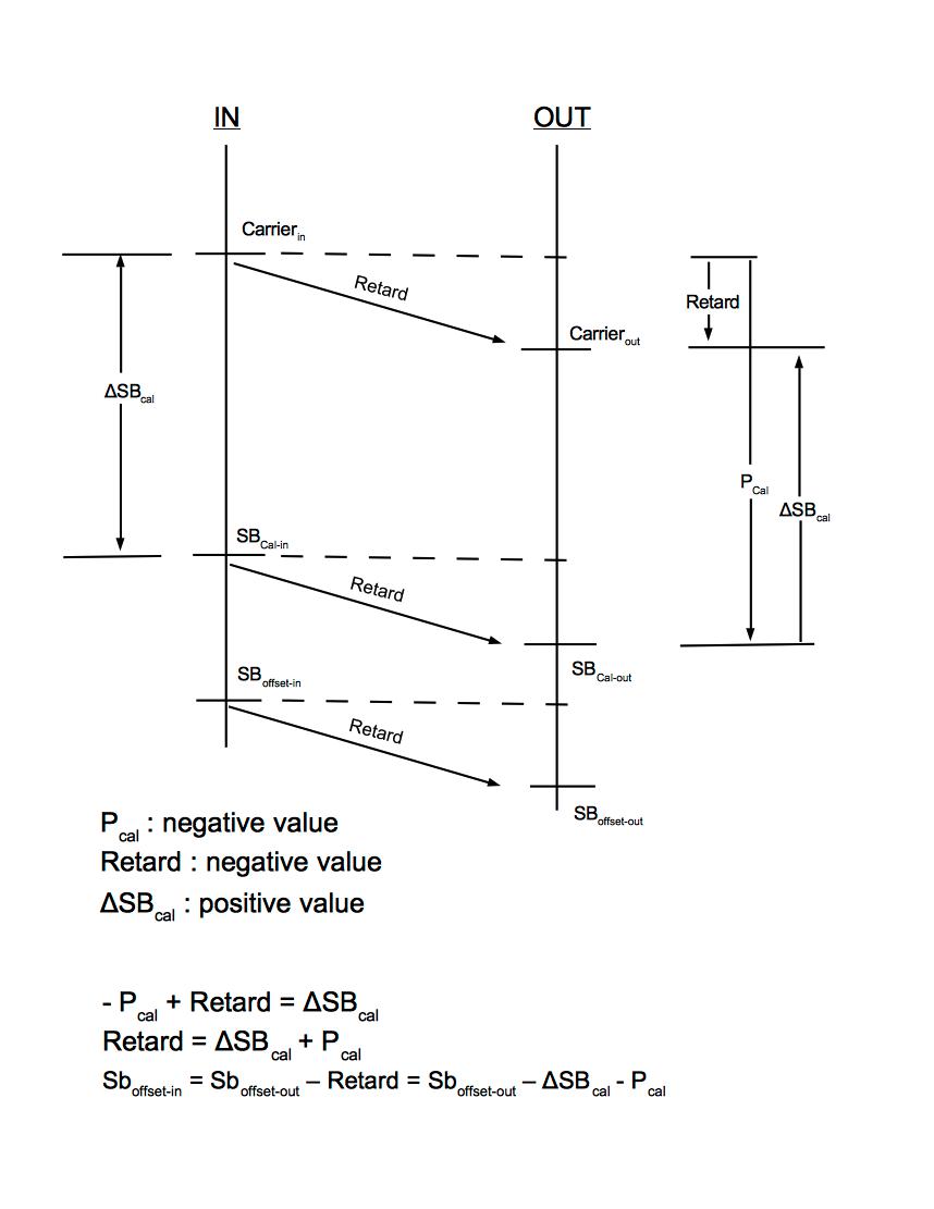
Figure 3 - The logic for the corrections using Delta_SB-cal and P-cal.

The HP11729C attenuates the signal levels at its inputs, which for the frequencies of interest is constant for a given setup. This attentuation value is represented as Retard in the figure.

On the left side of the figure is shown 3 signal levels that play a role in the correction mathematics. These are the Carrier input (Carrier_in), the sideband value for the calibration signal (SB_Cal-in) and the sideband value for a particular frequency offset (SB_offset-in). Each of these signals is attenuated in amplitude at the output side of the HP11729C. While the Carrier output (Carrier_out) is shown in the figure, its value is not measureable, since the double balanced mixer in the HP11729C executes carrier suppression.

The calibration levels (SB_Cal-in and SB_Cal-out) are both available, but the offset level SB_offset-in is not. Only SB_offset-out is measured. The goal is to use Carrier_in, SB_Cal-in, SB_Cal-out and SB_offset-out to compute SB_offset-in.

The strategy is to compute Retard and subtract it from SB_offset-out to get SB_offset-in. Delta_SB-cal equals Carrier_in minus SB_Cal-in and P-cal equals SB_Cal-out. As derived in the figure, Retard equals Delta_SB-cal plus P-cal. Therefore, SB_offset-in equals SB_offset-out minus Delta_SB-cal minus P-cal, which is the computation carried out in step 13 .

The subtraction of 6 dB from the measured phase noise power levels is justified in Appendix A (pg. 35) of HP product note 11729B-1. The derivation there is straight forward and so is not duplicated here.

Both the corrections section of the HP11729C Operating and Service Manual: pg. 3-21 and HP product note 11729B-1: pg. 25 note that for offset frequencies inside the loop bandwidth, a correction is necessary to the corresponding power levels, since they are attenuated. This is discussed on page 11 of the 11729B-1 product note in the second and third paragraphs. The attenuation is illustrated by an example shown in Figure 3.10.

The product note provides a formula for computing loop bandwidth when the HP11729C is used with an HP8662A. However, the test setup described here does not use an HP8662A; it uses a Wenzel HF-ONYX-IV, which has different characteristics than the HP8662A. So, it is necessary to derive the correct formula for loop bandwidth when using a Wenzel HF-ONYX-IV with the HP11729C.

Fortunately, Appendix B of the product note provides the necessary algebra to derive this quantity (pp. 37-38). The derivation uses 6 defined quantities:

K_d = Phase slope or phase detector gain factor of the mixer (volts/rad).

K_o =  VCO (EFC) slope (Hz/volt)

F = HP11729C Lock Bandwidth Factor

K_a(s) = loop amplifier gain

N = multiplication factor when a frequency band other than 5-1280 MHz is used. For this test setup, N =1.

s = 2*PI*j*f (Hz), where f=offset frequency.

On page 38, it states that K_d * K_a * K_o = 10^-3. Whereas the values of K_d and K_a are not given, on page 3-21 of the HP11729C Operating and Service Manual (under NOTE in the first paragraph), the value of K_o(HP8662A) is given as 10^-1 Hz/Volt. The Wenzel HF-ONYX-IV specification indicates a tuning range over 0-10V of +/- 10^-6, which for a 10 MHz oscillator translates to a range of +/- 10 Hz. Since the HP11729C EFC tuning signal bounds are +/- 10V, this means the Wenzel slope, K_o(Wenzel), when used with an HP11729C is 20Hz/20Volts = 1Hz/V (NB: a resistor divider network changes the Wenzel EFC range from 0-10V to +/- 10V). This is 10 times the value of K_o(HP8662A). Therefore, when using the Wenzel as Reference Oscillator, K_d * K_a * K_o = 10^-2.

This means the loop bandwidth of the HP11729C/Wenzel phase detector configuration equals F/10²]. For example, when using a Lock Bandwidth Factor of 100, the loop bandwidth equals 1 Hz.

The corrections for offsets inside the loop bandwidth are derived according to the instructions given on page 26 of the product note. However, if quadrature lock is obtained using a Lock Bandwidth Factor of 100 or less, no "inside the loop bandwidth" corrections are necessary.

[dnessett]

I have spent the last 2 months attempting to eliminate the 60Hz harmonic spurs apppearing in the output of my HP11729C. Those interested in the details can read the message thread that begins on Jan 11 (message #101757) on the HP-Agilent-Keysight-equipment@groups.io mail list (the whole thread can be accessed using the following link 60 Hz harmonic spurs on the HP11729C). Be forwarned, this is a long conversation, but there is useful information in it.

The conclusion of this discussion was the 60Hz and harmonic spurs were caused by the fan on the 11729C. After much discussion, I replaced the fan with a modern one (see the complete description of how to do this in this message). Unfortunately, while the fan replacement reduced the 60 Hz spur by about 12-13 dB, it increased the power of the 120 Hz and 240 Hz spurs by about 16 dB (see complete analysis here). So, replacing the fan did not solve the original problem.

Nevertheless, in the process of attacking it, I changed the procedure I use to measure phase noise using the phase detection mode of the 11720C. To ensure there is clairity in the interpretation of future results of my phase noise measurements, I document these changes here.

First, I now use a makeshift faraday cage to isolate the Oscillator under test from stray EMI. Following a suggestion by Leo Bodnar, I built the faraday cage out of a biscuit tin (Note: for those unfamiliar with non-US english, biscuit in UK english = cookie in US english. However, you will rarely if ever find cookies in the US packaged in a tin. I had to purchase some ginger snaps from Sweden at Cost Plus World Market to obtain the necessary hardware.)

Figure 1 shows the faraday cage opened to display how the oscillator fits into it. Note the use of plastic wrap to protect the electronics from shorting against the biscuit tin.


Figure 1 - Faraday cage opened

Figure 2 shows the faraday cage with the lid in place. At the top of the biscut tin are the connecting cables that feed the oscillator power and route the oscillator signal from it.


Figure 2 - Faraday cage closed

Second, in order to eliminate the possibility that the power source of either the oscillator under test or the reference oscillator is leaking 60 Hz + harmonics into the oscillators, I now power both using a battery. For 5 V oscillators, I use a 10000mAh ROMOSS Universal Power Bank. For 12 V oscillators I use a Talentcell Rechargeable 6000mAh Li-Ion Battery Pack.

Third, since my attempt to clean up 60 Hz + harmonic spurs by fixing the 11729C hardware failed, I now use software to remove non-stochastic spurs from phase noise plots. Fortunatley, Octave has a ready made routine for this in the signal pkg - medfilt1. Documentation is here. This routine uses a moving average replacement algorithm that replaces a data point by the median (not the mean) of the points in a window of size n around this point. It is eminently suited for spur removal in spectrum plots.

For example, figure 3 shows the 60 Hz and harmonic spurs in a plot of the output of the 11729C analyzing a Connor-Winfield HO100-61005SV low phase noise oscillator. (Recall that the output of the 11729C is not the phase noise of the device. Several corrections are required to this data to produce the phase noise of the oscillator.) Note the prominent 60 Hz and harmonics spurs in the spectrum plot.


Figure 3 - Plot of 11729C output for a Connor-Winfield HO100-61005SV low phase noise oscillator

Figure 4 shows the same output plot with the output of medfilt1 superimposed in red.


Figure 4 - Plot of 11729C output for a Connor-Winfield HO100-61005SV low phase noise oscillator with the output of medfilt1 superimposed in red

For reference, the data produced by the PicoScope 4262 uses ~20 mHz bins. So, each Hz bin comprises about 50 of these smaller bins. Therefore, I used a window of 100 to average the raw data over about 2 Hz.

One thing to note is the filtered data (i.e., the medfilt1 output) doesn't work well at very low Hz values. The reason for this is the window gets cut off at the left edge. There are two ways to implement this cut off in medfilt1. You can artifically zero fill the window out on the left to restore a window of 100 points. Alternatively, you can truncate the window and reduce the number of points in it.

Of these two options, truncate is the most appropriate for this application, since zero filling the window effectively makes the data to the left of 0 Hz equal to 0 dBc/Hz (technically 0 dBc/20mHz). This biases the result and raises the average above the expected value for low Hz power.

On the other hand, truncate also produces biased results. At very low frequencies the power is rising very fast. As you reduce the number of points in the window, the median no longer represents a unbiased estimate of the actual power at a particular Hz value. As is seen in the figure, the lower power values tend to dominate the median computation and the output artifically displays a value lower than what would be expected.

So, the filtered output is acceptiable down to 2 Hz, but below this value is not a true representation of the output. Imposing a conservative saftey margin, the filtered results probably should not be used for Hz values between 1-10 Hz.

There is a problem with simply showing the filtered phase noise, eliminating the spurs. For the Connor-Windfield oscillator, 60 HZ + harmonic spurs are the only ones with significant power. However, other oscillators have spurs unrelated to 60 Hz. For example, The Bliley NV47A1282 phase noise spectrum is cluttered with spurs unrelated to 60 Hz (see Figure 5).


Figure 5 - Plot of phase noise for a used Bliley NV47A1282 oscillator

It isn't clear what causes these spurs, but obviously eliminating them obscures the potential problems that might occur when employing such a used oscillator in an application. I plan on retaining the information these spurs convey by using the following two point strategy. First, I will rerun the Bliley oscillator phase noise tests using my 11729C with its upgraded fan and also using batteries to power the oscillators. Second, when displaying a phase noise plot, I will always superimpose the spur removed plot over the plot of the raw phase noise data. This will show where the spurs were removed and afford the observer an opportunity to interpret the causes of the spectrum spurs.

Finally, I am using one other modification to my prior described test setup. My Rigol DG1022 went belly up and so I have purchased a Siglent 40 MHz SDG 2042X function generator. I will not update the instructions how to use this new function generator to calibrate the 11729C when using a particular oscillator, since these effectively do not change. There might be one or two minor differences (e.g., how to connect an external 10 MHz signal to the function generator), but the translation from one function generator to the other should be obvious.