I'm not sure about how to do that spectrograph. I can plot one, but since we are phaseshifting, the frequencies of the waves won't change, so the spectrogram will be flat. Maybe a phase vs time graph?
Anyway, I believe your idea of thinking about specific frequencies is okay, and you don't need to overcomplicate things. I'll try to explain again, using a different argument. The explanation should be split in two parts: first, meaning of phase vs group delay. Second, how do you interpret that intuitively. Some heavy graphs to come: this time I'm doing them in python and including source at the ending.
First: phase shift versus group delay.
Having a filter with phase shift of 1 rad at 50Hz means that a pure 50Hz wave passing through that filter will experience a phase shift of 1 radian. Note that this says
absolutely nothing about what happens at other frequencies: this filter could have arbitrary phase shifts at 51Hz, 100Hz, or 17Hz.
Group delay is a derivative: the ratio of phase shift relative to frequency. Instead of seconds, think that group delay is measured in radians per Hz, rad/Hz. If you have a group delay of 1 rad/Hz at 50Hz, that means that at 51Hz you will have 1 more radian of phase shift than at 50Hz. At 52Hz you will have 2 rads more than at 50Hz. And at 49Hz you will have 1 rad less of phase shift than at 50Hz.
Group delay tells you how phase shift changes when you deviate from the frequency where you measure it.Joining both concepts: if you have a phase shift of 2 radians at 50Hz and a group delay of 3 rad/Hz, that means phase shifts of: 2 rad @ 50Hz, 5rad @ 51Hz, 8rad @ 52Hz, -1 rad @ 49Hz, -4 rad @ 48 Hz, etc.
It is important to note the following: if you have a filter with zero phase shift at 50Hz, and with 100 rad/Hz group delay at 50Hz. If you pass a pure 50Hz wave through that filter, the wave will be... unaltered. A 51Hz sinewave would be shifted 100rads, and a 49Hz one -100rads, but the 50Hz wave is unaltered.
So, phase shift gives you the phase at an specific frequency. If you also know group delay, it gives you the phase shift at nearby frequencies.
Note that group delay, by itself, is not enough to determine phase shift. You need the phase shift at a given frequency for reference. So, if you only know group delay, even if you ignore phase shift, what does that mean? This is for part 2.
Second: Intuitive meaning of group delay.
The idea that group delay is how the "envelope" of a carrier wave is phase shifted, while the carrier remains unaltered, is correct. Let us try to visualize that. By carrier wave we mean the pure frequency at which you measure the group delay. By envelope we mean the nearby frequencies, that will experience different phase shifts the farther they are from the carrier (because that's what group delay means, more away in frequency, more phase deviation).
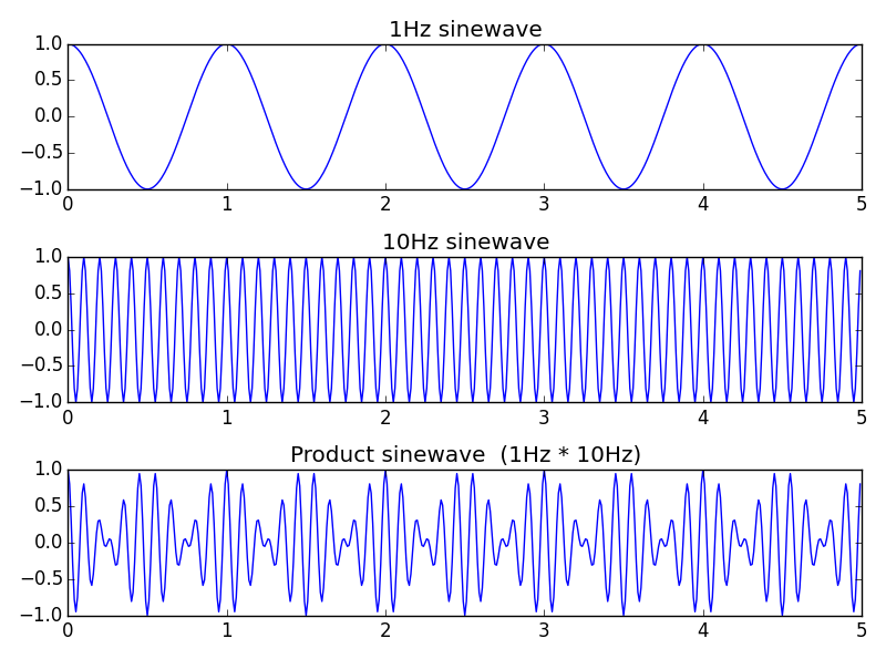
Imagine that you have a pure 10Hz wave (not 50Hz anymore, in the graphs lower frequencies look clearer). Let us create a waveform that has an "envelope" at 10Hz. The easiest way is the following: we get a 10Hz wave and multiply it by a 1Hz wave. The result is a 10Hz wave "filling up" the shape of the 1Hz wave.
This product wave we have obtained is not a simple sinewave, so it's natural to ask ourselves what's its spectrum. Here high school trigonometry comes in our help. Let's see, a 10Hz (forget the pi's!) sinewave is \$\cos(10 t)\$ and a 1Hz sinewave is \$\cos(t)\$. So the product wave is \$\cos(10t)\cos(t)\$.
Remember the cosine addition laws? \$\cos(a+b) = \cos a\cos b - \sin a\sin b\$ and \$\cos(a-b) = \cos a\cos b + \sin a\sin b\$. If you add both relations, you obtain:
\$\cos(a+b) + \cos(a-b) \ = \ 2\cos a\cos b\$
What is relevant of this relation is that it turns a product of cosines into a sum of
pure cosines. If you make a=10t, b=t, you get:
\$\cos(11t) + \cos(9t) \ = \ 2\cos 10t\cos t\$
In other words, the spectrum of our product wave has components at 9Hz and 11Hz, and none at 10Hz. Let us check that:

Notice that the added wave goes from -2 to 2? It's that pesky factor of two in the cosine law. Let's compare the product and addition waves to be sure:

Okay, they match (save for the 2x factor). Now we are ready to understand why group delay operates on envelopes. Notice:
-> Since our waveform has no fourier component at 10Hz, it is unaffected by any phase shift at 10Hz.
-> Since out waveform has fourier components near 10Hz, it is affected by group delay at 10Hz.
Okay, our waveform is affected by group delay. But affected, how?
Imagine we have a filter with no phase shift at 10Hz, but with group delay of 1 rad/Hz. This means that the component of our waveform at 9Hz will be shifted by -1rad, and the component at 11Hz will be shifted by 1rad. Remember the cosine law? If we write it in reverse:
\$\cos a + \cos b \ = \ 2\cos\frac{a+b}{2}\cos\frac{a-b}{2}\$
\$\cos(11t+1) + \cos(9t - 1) \ = 2\ cos\frac{11t+1+9t-1}{2}\cos\frac{11t+1-9t+1}{2} \ = \ 2\cos 10t \cos(t+1) \$
The 10Hz "carrier" part is unaltered, while the 1Hz "envelope" part is shifted by 1 radian! This is what group delay does to nearby frequencies: it
coherently phase shifts them with respect to the center frequency.
Below there are graphics for the 1 rad/Hz delay, and also a 2 rad/Hz delay:

There you can see that the carrier is coherently delayed by the given angle: the whole wavepacket is delayed without losing it shape.
As promised, the source code for the images. It requires python with numpy and matplotlib.
import numpy as np
import matplotlib.pyplot as plt

t = np.arange(0.0, 5.0, 0.01)
s10 = np.cos(2*np.pi*10*t)
s1 = np.cos(2*np.pi*1*t)
sp = s1*s10

# 1Hz, 10Hz, product.
fig, (sub1, sub2, sub3) = plt.subplots(nrows=3)
sub1.set_title("1Hz sinewave")
sub2.set_title("10Hz sinewave")
sub3.set_title("Product sinewave  (1Hz * 10Hz)")
sub1.plot(t, s1)
sub2.plot(t, s10)
sub3.plot(t, sp)
plt.tight_layout()
plt.show()

# 9Hz, 11Hz, addition.
fig, (sub1, sub2, sub3) = plt.subplots(nrows=3)
s9 = np.cos(2*np.pi*9*t)
s11 = np.cos(2*np.pi*11*t)
sadd = s9 + s11
sub1.set_title("9Hz sinewave")
sub2.set_title("11Hz sinewave")
sub3.set_title("Added sinewaves (9Hz + 11Hz)")
sub1.plot(t, s9)
sub2.plot(t, s11)
sub3.plot(t, sadd)
plt.tight_layout()
plt.show()

# Comparison.
fig, (sub1, sub2) = plt.subplots(nrows=2)
sub1.set_title("Product sinewave  (1Hz * 10Hz)")
sub2.set_title("Added sinewaves (9Hz + 11Hz)")
sub1.plot(t, sp)
sub2.plot(t, sadd)
plt.tight_layout()
plt.show()

# Apply 1 rad/Hz [s] and 2 rad/Hz group delays.
fig, (sub1, sub2, sub3) = plt.subplots(nrows=3)
sub1.set_title("Normal wave (9Hz + 11Hz)")
sub2.set_title("1 rad/Hz delayed wave")
sub3.set_title("2 rad/Hz delayed wave")
sub1.plot(t, sadd)
sdel1 = np.cos(2*np.pi*9*t-1) + np.cos(2*np.pi*11*t+1)
sub2.plot(t, sdel1)
sdel2 = np.cos(2*np.pi*9*t-2) + np.cos(2*np.pi*11*t+2)
sub3.plot(t, sdel2)
plt.tight_layout()
plt.show()


